GridWorld

First Example

This is the example 3.5 from [S.Sutton2018].

For a full example, see how to build this example from the S&B book:

import numpy as np
from emdp import actions
import emdp.gridworld as gw

def build_SB_example35():
    """
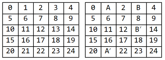
    Example 3.5 from (Sutton and Barto, 2018) pg 60 (March 2018 version).
    A rectangular Gridworld representation of size 5 x 5.

    Quotation from book:
    At each state, four actions are possible: north, south, east, and west, which deterministically
    cause the agent to move one cell in the respective direction on the grid. Actions that
    would take the agent off the grid leave its location unchanged, but also result in a reward
    of −1. Other actions result in a reward of 0, except those that move the agent out of the
    special states A and B. From state A, all four actions yield a reward of +10 and take the
    agent to A'. From state B, all actions yield a reward of +5 and take the agent to B'
    """
    size = 5
    P = gw.build_simple_grid(size=size, p_success=1)
    # modify P to match dynamics from book.

    P[1, :, :] = 0 # first set the probability of all actions from state 1 to zero
    P[1, :, 21] = 1 # now set the probability of going from 1 to 21 with prob 1 for all actions

    P[3, :, :] = 0  # first set the probability of all actions from state 3 to zero
    P[3, :, 13] = 1  # now set the probability of going from 3 to 13 with prob 1 for all actions

    R = np.zeros((P.shape[0], P.shape[1])) # initialize a matrix of size |S|x|A|
    R[1, :] = +10
    R[3, :] = +1

    p0 = np.ones(P.shape[0])/P.shape[0] # uniform starting probability (assumed)
    gamma = 0.9

    terminal_states = []
    return gw.GridWorldMDP(P, R, gamma, p0, terminal_states, size)

where P is the transition model \(P: \mathcal{S}\times\mathcal{A}\times\mathcal{S}\mapsto \mathbb{R}\), R is the reward map \(r: \mathcal{S}\times\mathcal{A}\mapsto\mathbb{R}\).

To actually use this there is a gym like interface where you can move around:

mdp = build_SB_example35()
state = mdp.reset()
next_state, reward, done, _ = mdp.step(actions.UP) # moves the agent up.

Plotting GridWorlds

from emdp.gridworld import GridWorldPlotter
from emdp import actions
import random

gwp = GridWorldPlotter(mdp.size, # 5
                       mdp.has_absorbing_state)
# alternatively you can use GridWorldPlotter.from_mdp(mdp)

# collect some trajectories from the GridWorldMDP object:

trajectories = []
for _ in range(3): # 3 trajectories
    trajectory = [mdp.reset()]
    for _ in range(10): # 10 steps maximum
        state, reward, done, info = mdp.step(random.sample([actions.LEFT, actions.RIGHT,
                                                            actions.UP, actions.DOWN], 1)[0])
        trajectory.append(state)
    trajectories.append(trajectory)

Now trajectories contains a list of lists of numpy arrays which represent the states. You can easily obtain trajectory plots and state visitation heatmaps:

import matplotlib.pyplot as plt

fig = plt.figure(figsize=(10, 4))
ax = fig.add_subplot(121)

# trajectory
gwp.plot_trajectories(ax, trajectories)
gwp.plot_grid(ax)

# heatmap
ax = fig.add_subplot(122)
gwp.plot_heatmap(ax, trajectories)
gwp.plot_grid(ax)

You will get something like this:

Customization

There is an interface to add walls and blockages to the gridworld.

import numpy as np
from emdp.gridworld.builder_tools import TransitionMatrixBuilder
from emdp.gridworld import GridWorldMDP

builder = TransitionMatrixBuilder(grid_size=5, has_terminal_state=False)
builder.add_grid([], p_success=1)
builder.add_wall_at((4, 2))
builder.add_wall_at((3, 2))
builder.add_wall_at((2, 2))
builder.add_wall_at((1, 2))

construct MDP and plot trajectories:

P = builder.P
R = np.ones((P.shape[0],P.shape[1]))
p0= np.ones((5,5))
p0[4,2] = 0
p0[3,2] = 0
p0[2,2] = 0
p0[1,2] = 0
p0 = (p0 / np.sum(p0)).reshape((5*5,))
mdp = GridWorldMDP(P,R,gamma=0.9,p0=p0,terminal_states=[],size=5)

from emdp.gridworld import GridWorldPlotter
from emdp import actions
import random

gwp = GridWorldPlotter(mdp.size, # 5
                    mdp.has_absorbing_state)
# alternatively you can use GridWorldPlotter.from_mdp(mdp)

# collect some trajectories from the GridWorldMDP object:

trajectories = []
for _ in range(30): # 30 trajectories
    trajectory = [mdp.reset()]
    for _ in range(100): # 100 steps maximum
        state, reward, done, info = mdp.step(random.sample([actions.LEFT, actions.RIGHT,
                                                            actions.UP, actions.DOWN], 1)[0])
        trajectory.append(state)
    trajectories.append(trajectory)

import matplotlib.pyplot as plt

fig = plt.figure(figsize=(10, 4))
ax = fig.add_subplot(121)

# trajectory
gwp.plot_trajectories(ax, trajectories)
gwp.plot_grid(ax)

# heatmap
ax = fig.add_subplot(122)
gwp.plot_heatmap(ax, trajectories)
gwp.plot_grid(ax)

Alternatively, you can use add_wall_between which creates a straight line of walls between two positions on the grid. So the following code will produce

from emdp.gridworld.builder_tools import TransitionMatrixBuilder
builder = TransitionMatrixBuilder(grid_size=5, has_terminal_state=False)
builder.add_grid([], p_success=1)
builder.add_wall_between((0,2), (1, 2))
builder.add_wall_between((3,2), (4, 2))
builder.add_wall_between((1,1), (1, 3))

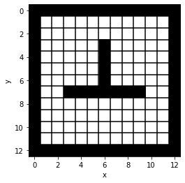
From String

from emdp.gridworld.txt_utilities import get_char_matrix, build_gridworld_from_char_matrix
from emdp.gridworld import GridWorldPlotter
import matplotlib.pyplot as plt

str_rows = """\
#############
#           #
#         g #
#     #     #
#     #     #
#     #     #
#     #     #
#  #######  #
#           #
#           #
#           #
#s          #
#############""".split('\n')

mdp, mdp_wall_locs = build_gridworld_from_char_matrix(get_char_matrix(str_rows))

plotter = GridWorldPlotter.from_mdp(mdp)

fig = plt.figure(figsize=(4, 4))
ax = fig.add_subplot(111)
plotter.plot_environment(ax, wall_locs = mdp_wall_locs, plot_grid = True)
plt.show()

References

S.Sutton2018

S.Sutton, Richard, and Andrew G.Barto. 2018. Reinforcement Learning: An Introduction. Second Edition. The MIT Press.